finite-element-code
This code computes a finite-element solution to boundary value problems of the form:
on some domain $\Omega$.
With $N$ nodes and basis functions $\phi(x,y)_{i=1,2,...,N}$ , our FEM solution takes the form:
$$\sum_{i=1}^{N} \alpha_i\;\phi_i(x,y)$$
where $\phi_i(x,y)$ are piece-wise linear 'pyramid-shaped' functions about node $i$.
Also, let $u = \alpha_1,\alpha_2,...,\alpha_i$. Then, $u$ is computed by $u=K^{-1}F$ where $K$ is the global stiffness matrix and $F$ is the global load vector.
By default, the code uses a structured triangular mesh, but this can be easily maniputed in user_input.m as demonstrated in Example 2.
Currently only supports Dirichlet boundary conditions (or homogenous Neumann BCs for the mixed case).*
Begin by initializing the problem in user_input.m.
rectangle_domain.m or circle_domain.m are used by default (see user_input.m).
Any other custom meshes will need to be imported manually.
Additionally, MESH is a Matlab triangulation object that stores two properties: Points and ConnectivityList.
When ready, run main_2d.m, which consists of the following steps:
user_input; //read problem input
psi = polyLagrange2D(p); //determine Lagrange shape functions of degree p = 1
[K,F]=element2D(psi,KofXY,BofXY,FofXY,MESH); //compute load/stiffness matrices
[K,F]=enforce2DBCs(K,F,KofXY,boundaryValues,boundaryNodes); //enforce boundary conditions
u=K\F;
trimesh(MESH.ConnectivityList,MESH.Points(:,1),MESH.Points(:,2),u); //plot solution
Example 1 (structured rectangular mesh):
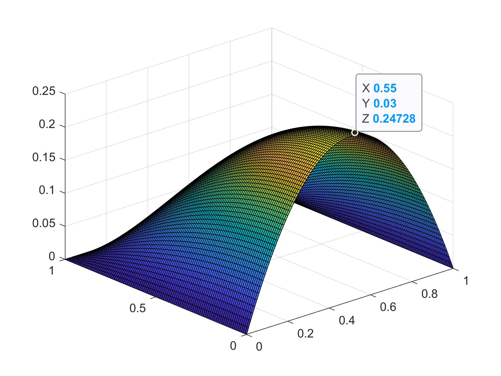
Solving
$$-\nabla^2u(x,y)+u(x,y) = \pi^2e^{-x}sin(\pi y) \text{ on the unit square } \Omega:[0,1]\times[0,1]$$
with Dirichlet boundary conditions
$$u(0,y) = sin(\pi y),\; u(x,1) = 0,\; u(1,y) = \frac{sin(\pi y)}{e},\; u(x,0) = 0$$
we obtain an exact solution of $u(x,y) = e^{-x}sin(\pi y)$ (left), compared to our FEM solution (right).
sin(piy)_exact.jpg)
sin(piy)_fem.jpg)
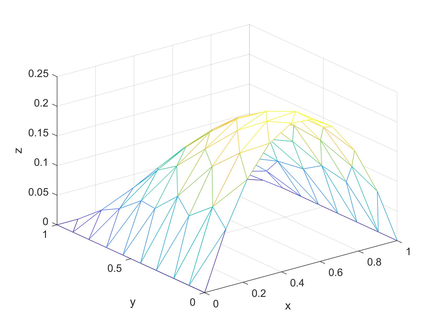
Example 2 (unstructured rectangular mesh):
Solving
$$-\nabla\cdot((1+xy^2)\nabla u(x,y)) = 2-3y^2-6x^3y^2+y^4+x^2(6y^2-2)+x(2+4y^2-4y^4)$$
with mixed boundary conditions
$$u(0,y) = u(x,1) = u(1,y) = 0,\; \frac{\partial u(x,0)}{\partial y} = 0 $$
we find our exact solution to be $u(x,y) = (x^2-x)(y^2-1)$ (left) and also an FEM solution, this time using an unstructured mesh (right).
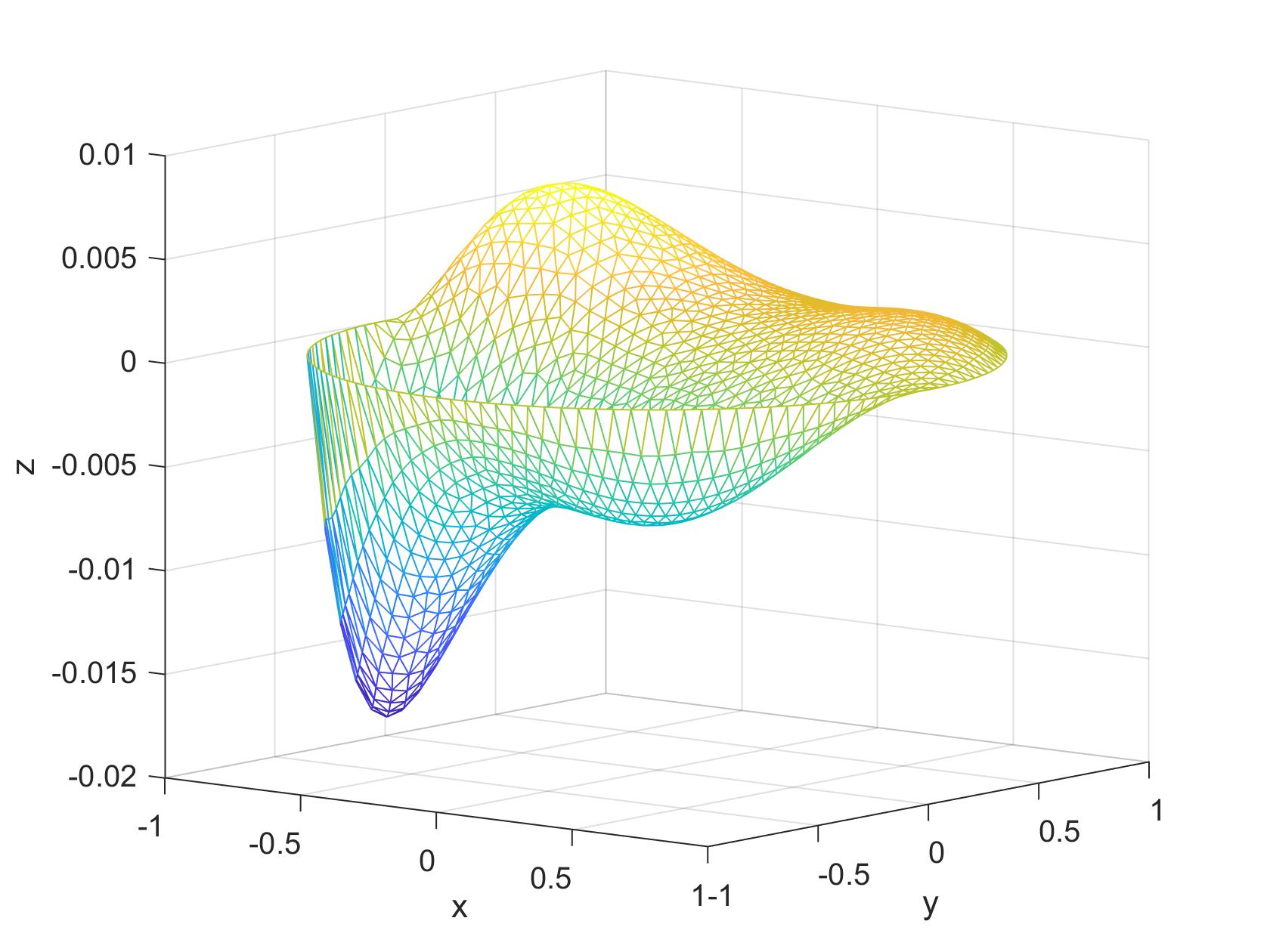
Example 3, 4 (circular mesh):
Solutions are also computable across circular domains: $$\Omega: \{(x, y) \in \Bbb R^2, \; x^2 + y^2 \le 1 \}$$ $$-\nabla\cdot((e^{x+y})\nabla u(x,y)) = x^2y\,, \quad u(x,y) = 0 \;\text{on}\; \partial\Omega$$
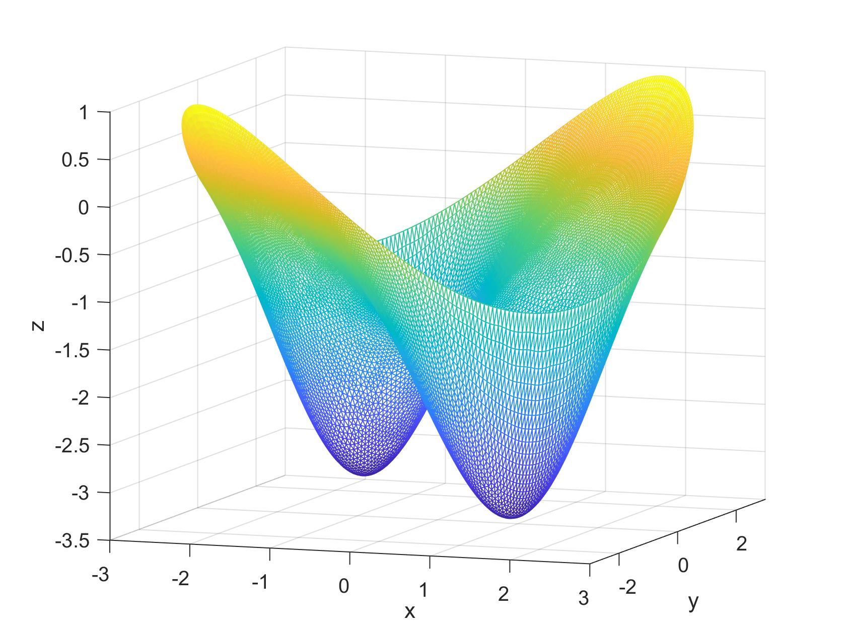
Example 5:
As discussed previously, this code is not limited to just rectangular/circular domains.
Any appropriately defined 2-D mesh with boundary conditions is computable.
Here are a few examples: $$\Omega: \{(x,y) \in \Bbb R^2, \; [(x-1)^2 + (y-1)^2 \ge 1/16] \land [0 \le x \le 2] \land [0 \le y \le 2]\}$$
$$-\nabla^2u(x,y) = 100sin(10xy)\,, \quad u(x,y) = 0 \;\text{on}\; \partial\Omega_1,\;u(x,y) = sin(3\theta) \;\text{on}\; \partial\Omega_2$$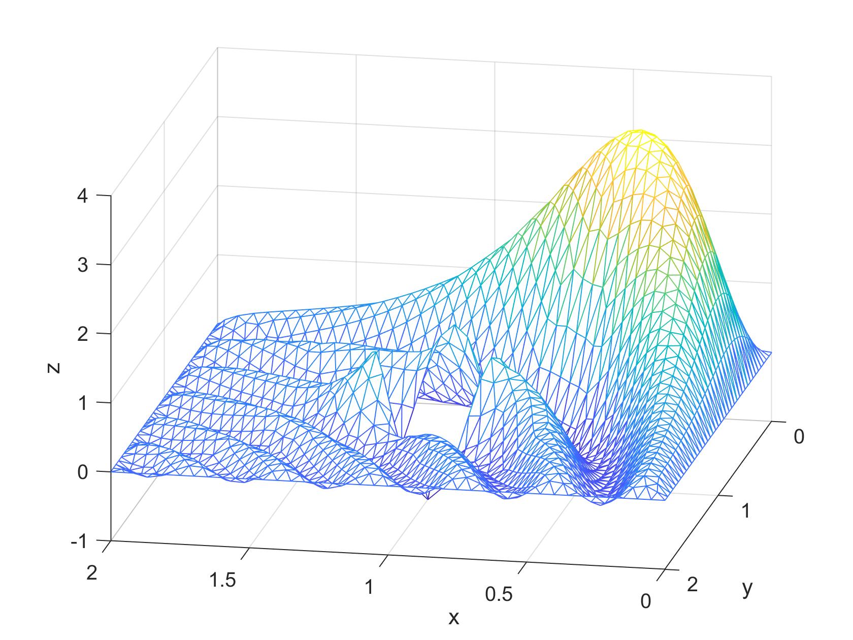
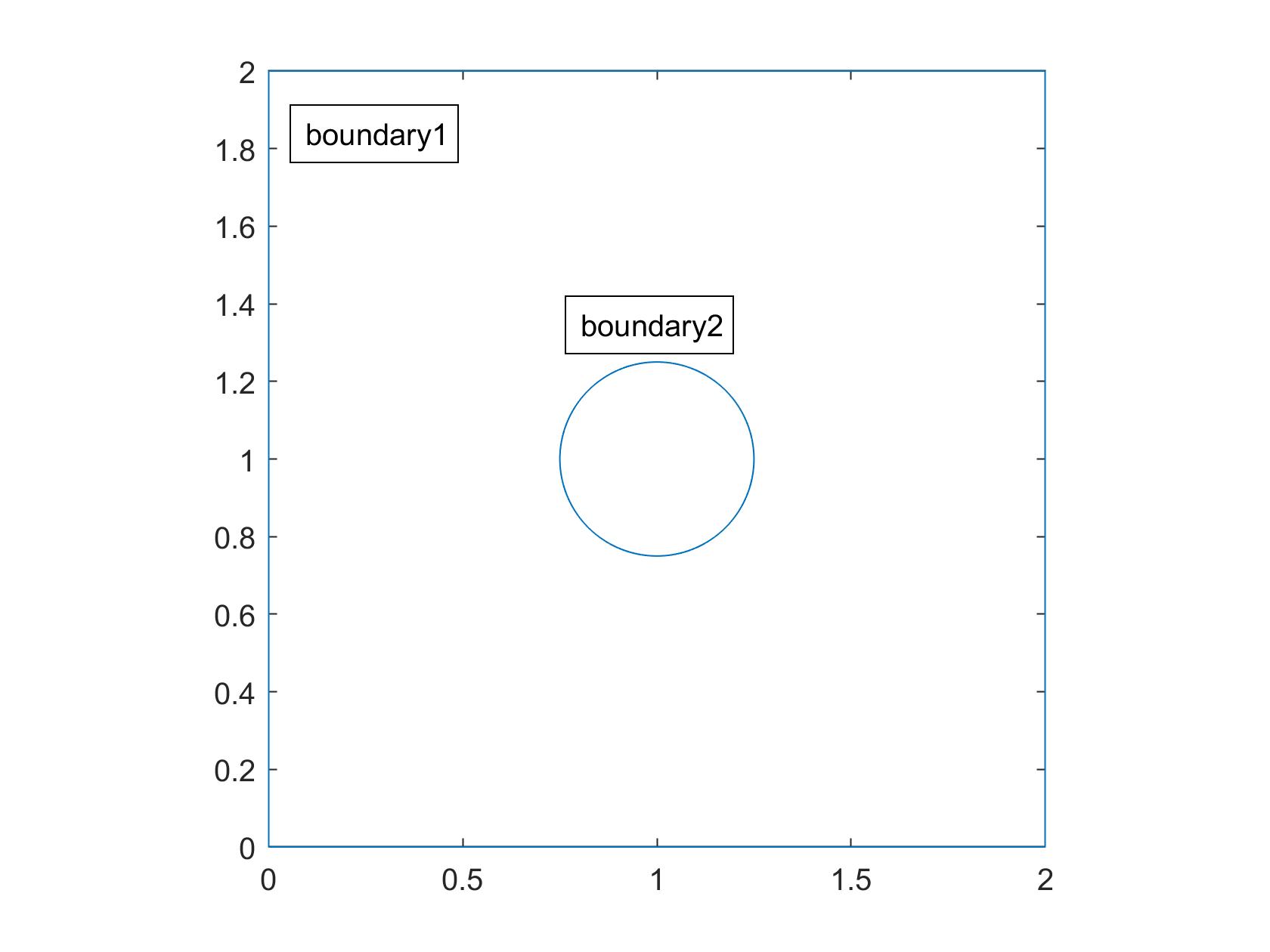
This mesh was created using Matlab's geometryFromEdges function. See custom_mesh1.m.
$$\Omega: \{(x,y) \in \Bbb R^2, \; [(x-2)^2+y^2 \ge 1.2^2] \land [(x-4)^2+(y-2)^2 \ge 1.2^2]$$$$\land [(x-2)^2+(y-4)^2 \ge 1.2^2] \land [x^2 + (y-2)^2 \ge 1.2^2] \land [0 \le x \le 4] \land [0 \le y \le 4]\}$$$$-\nabla\cdot([(x-2)^2y+(y-2)^2]\nabla u(x,y)) = (x-2)(y-2)\,, \quad u(x,y) = 0 \;\text{on}\; \partial\Omega$$
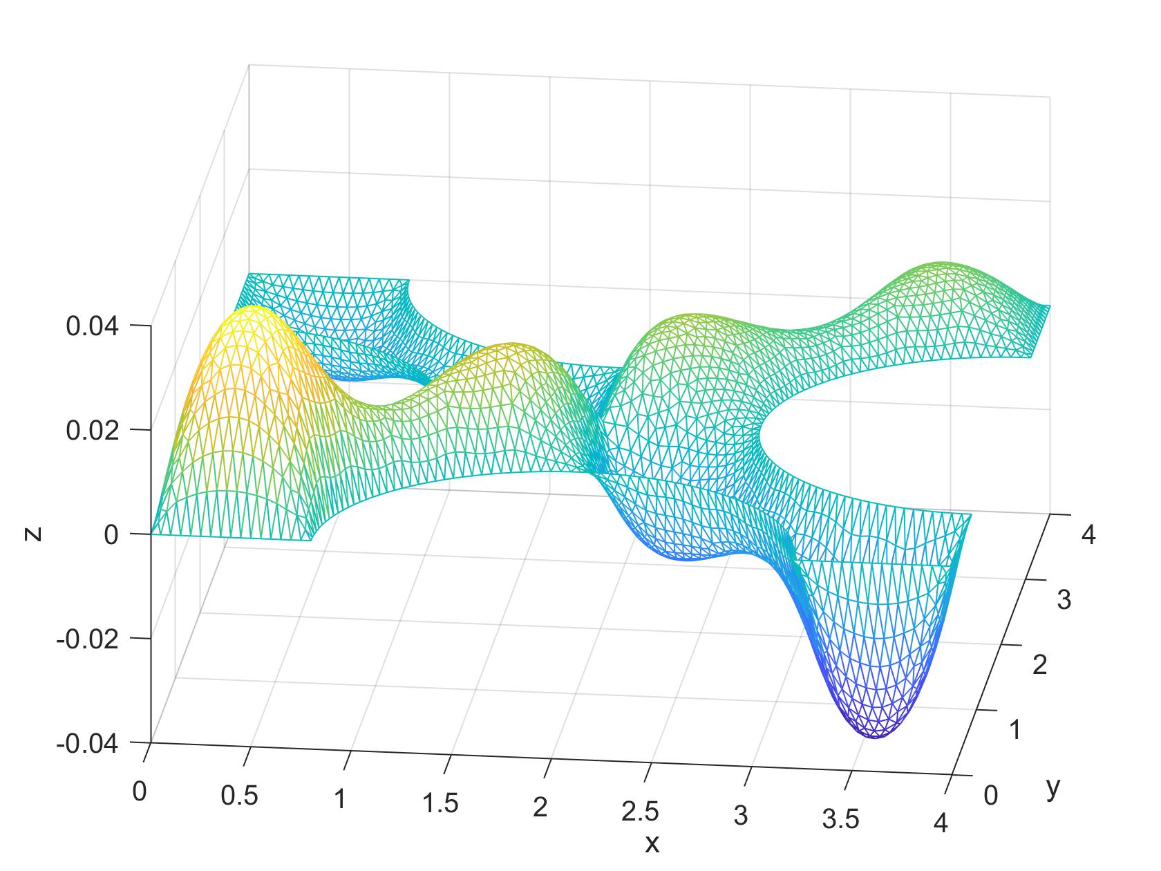
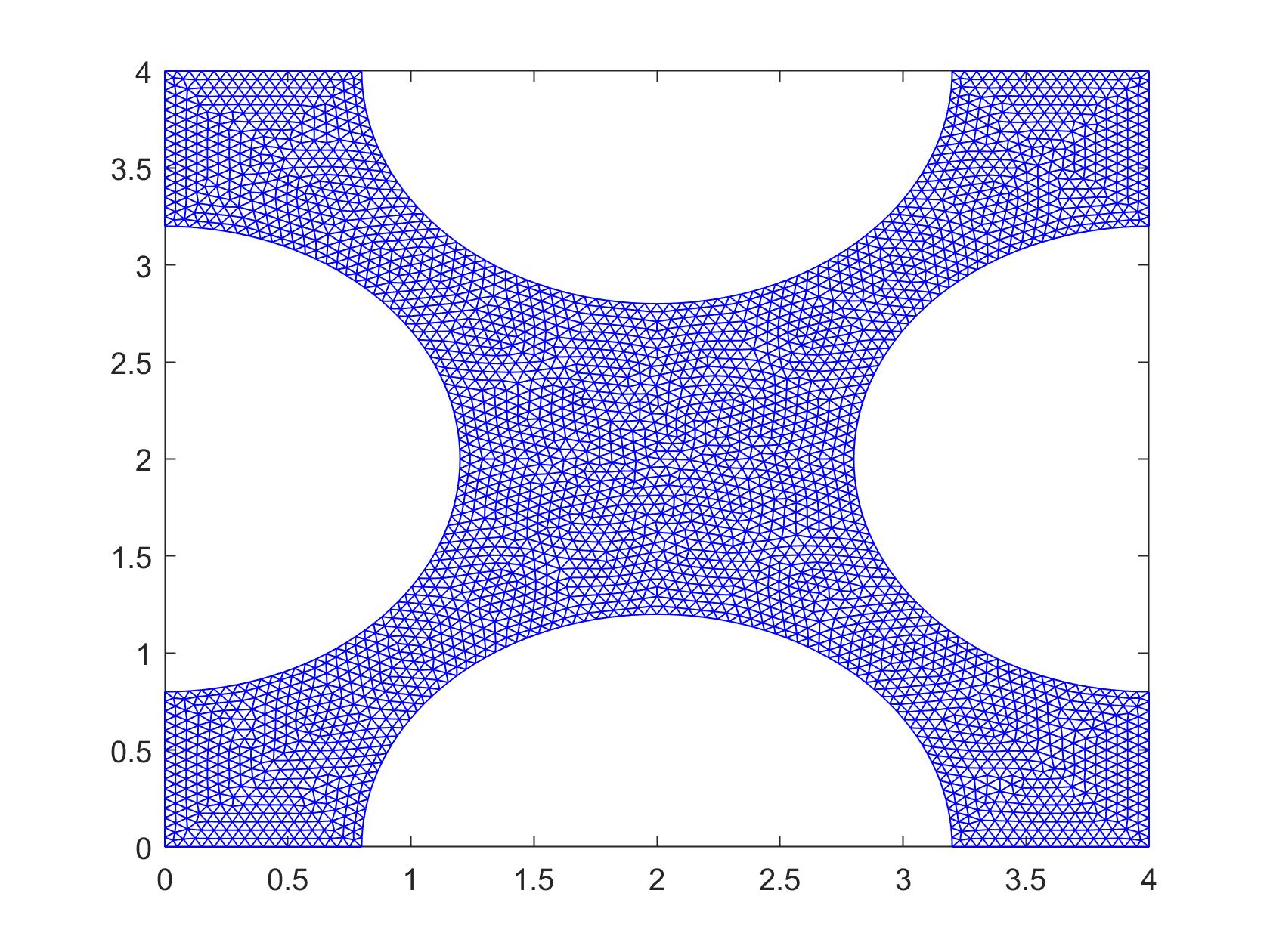
See custom_mesh2.m.